GRACE TECHNICAL REPORTS
Trace-based Approach to Editability and
Correspondence Analysis for Bidirectional
Graph Transformations
Soichiro Hidaka
Martin Billes
Quang Minh Tran
Kazutaka Matsuda
GRACE-TR 2015–04
February 2015
CENTER FOR GLOBAL RESEARCH IN
ADVANCED SOFTWARE SCIENCE AND ENGINEERING
NATIONAL INSTITUTE OF INFORMATICS
2-1-2 HITOTSUBASHI, CHIYODA-KU, TOKYO, JAPAN
Correspondence Analysis for Bidirectional
Graph Transformations
⋆Soichiro Hidaka1, Martin Billes2, Quang Minh Tran3, and Kazutaka Matsuda4
1
National Institute of Informatics, Japan
2
Augsburg University, Germany
3
Daimler Center for IT Innovations, Technical University of Berlin, Germany
4
The University of Tokyo
Abstract. Bidirectional graph transformation is expected to play an important role in model-driven software engineering where artifacts are often refined through compositions of model transformations, by propa-gating changes in the artifacts over transformations bidirectionally. How-ever, it is often difficult to understand the correspondence among ele-ments of the artifacts such as to which part in the source an edit on the view is to be propagated. It is equally hard to predict whether an edit is propagable to the source, if the edit affects other parts in the target, or where in the transformation should be changed to accommodate the edit. These issues are critical for more complex transformations. In this paper, we propose an approach to analyzing the above correspondence as well as to classifying edges according to their editability on the target, in a compositional framework of bidirectional graph transformation. These are achieved by augmenting the forward semantics of the transforma-tions with explicit correspondence traces. By leveraging this approach, it is possible to solve the above issues, without executing the entire back-ward transformation. We demonstrate the effectiveness of our approach via GUI using non-trivial transformations.
Keywords: Bidirectional Graph Transformation, Traceability, Editabil-ity
⋆This is a full version of the paper submitted to the 8th International Conference on
1
Introduction
Bidirectional transformations has been attracting interdisciplinary stud-ies [7,21], for example as the view-update problem in the database community [3,8] and more recently in the programming language community [11,4]. In model-driven software engineering where artifacts are often refined through compositions of model transformations, bidirectional graph transformation is expected to play an important role, because it enables us to propagate changes in the artifacts over transformations bidirectionally. Other usage of bidirectional model transformation could be distilling a complicated model down to just the features a certain stakeholder is interested in, or converting information to a different platform, such as classes to relational databases.
G
SG
VF
G
′V
edit
G
′S
B
A bidirectional transformation consists of forward (F) and backward (B) transformations [7,21]. F takes a source model (here a source graph [16,17]) GS and
transforms it into a view graph GV. B takes an
up-dated view graph G′V and returns an updated source graph G′S, with possibly propagated updates.
In many, especially complex transformations, it is not immediately apparent whether a view edge has its origin in a particular source edge or a part in the transformation, and what that part is. Thus, it is not easy to tell where edits to the view edge are propagated back too. In particular, backward transformation rejects updates if (1) the label of the edited view edge appears as a constant of the transformation, (2) a group of view edges are edited inconsistently or (3) edits of view edges lead to changes in branching behavior in the transforma-tion. If a lot of edits are made at once, it becomes increasingly difficult for the user to predict whether these edits are accepted by backward transformation. Bidirectional transformations are known for being hard to comprehend and pre-dict [10]. Two features are desirable: 1) Explicit highlighting of correspondence between source, view and transformation 2) Classification of artifacts according to their editability. This way, prohibited edits leading to violation of predefined properties can be recognized by the user early.
view edges that cannot be inconsistently modified to different label names are highlighted in green.
There is some existing work with similar objectives. For tracing, Van Amstel et al. [2] proposed the visualization of traces, but in the unidirectional model transformation setting. For classification of elements in the view, Matsuda and Wang’s work [22] in the context of extension of semantic approach [27] to general bidirectionalization, is also capable of similar classification, while we reserve opportunities to recommend variety of consistent changes for more complex branching conditions. In addition, our approach can trace between nodes of the graph, not just edges.
The rest of the paper is organized as follows: Section 2 overviews our moti-vation and goal with a running example. The simplicity of the example is for the sake of explanation, and we have more involved examples related to software en-gineering in our project website mentioned in Section 6. Section 3 summarizes the semantics of our underlying graph data model, core graph language UnCAL [5], and its bidirectional interpretation [14]. Section 4 introduces an augmented se-mantics of UnCAL to generate trace information for the correspondence and editability analysis. Section 5 explains how the augmented forward semantics can be leveraged to realize correspondence and editability analysis. An imple-mentation is found at the above website. Section 6 describes how the proposed mechanisms in the preceding sections are integrated in GRoundTram.5Section 7 discusses related work, and Section 8 concludes the paper with future work.
2
Motivating Example
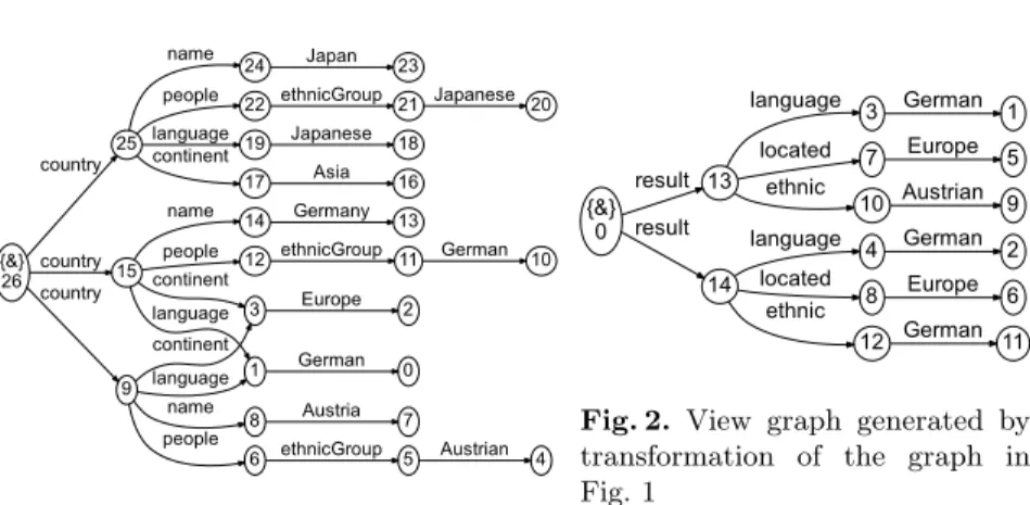
This section exemplifies the importance of the desireble features mentioned in Sect. 1. Let us consider the source graph in Fig. 1 consisting of fact book informa-tion about different countries, and suppose we want to extract the informainforma-tion for European countries as the view graph in Fig. 2. This transformation can be written in UnQL (the surface language of our target language UnCAL) as below.
select{result:{ethnic: $e, language: $lang, located: $cont}}
where{country:{name:$g, people:{ethnicGroup: $e}, language: $lang, continent: $cont}}in$db,
{$l:$Any}in$cont, $l= Europe
Listing 1.1.Transformation in UnQL
In the view graph (Fig. 2), three edges have identical labels “German” (3,German,1), (4,German,2) and (12,German,11), but have different origins in the source graph and are produced by different parts in the transformation. For example, the edge ζ= (3,German,1) is the language of Germany and is a
5
{&} 26 25 country 15 country 9 country 24 name 22 people 19 language 17 continent 23 Japan 21
ethnicGroup Japanese 20 18 Japanese 16 Asia 14 name 12 people 3 continent 1 language 13 Germany 11 ethnicGroup 10 German 8 name 6 people continent language 7 Austria 5
ethnicGroup Austrian 4 2
Europe 0 German
Fig. 1.Example source graph
{&} 0 13 result 14 result 3 language 7 located 10 ethnic 4 language 8 located 12 ethnic 1 German 2 German 5 Europe 6 Europe 9 Austrian 11 German
Fig. 2. View graph generated by transformation of the graph in Fig. 1
copy of the edge (1,German,0) of the source graph (Fig. 1). On the other hand,
ζ has nothing to do with the edge (11,German,10) of the source graph despite identical labels. This later edge denotes the ethnic group instead. In addition,ζ
is copied by the graph variable $lang in theselectpart of the transformation. Other graph variables and edge constructors do not participate in creatingζ. It would be much easier for the user to understand, if the system visually highlights corresponding elements between source graph, view graph and transformation to increase comprehensibility.
In this example, the non-leaf edges of the view graph (“result”, “located”, “language” and “ethnic”) are constant edges in the sense that they cannot be modified by the user in the view. The user may not be aware of this and try to rename “located” to “location”, but backward transformation rejects this change. Ideally, the system should make such constant edges easily recognizable to prevent the edits in the view and guide the user to make an edit to the constant in the transformation instead.
In another scenario, the user decides that the language of Germany should better be called “German (Germany)” and the language of Austria be called “Austrian German” and thus rename the view edges (3,German,1) and (4,German,2) to (3,German (Germany),1) and (4,Austrian German,2) accordingly. However, the backward transformation rejects this modification because these two view edges originate from the language “German” in a single edge of the source graph. The backward propagation of two edits would conflict at the source edge. The user may not realize this until the rejection. Ideally, the system would highlight groups of edges that could cause the conflict, and would prohibit triggering the backward transformation in that case.
are very difficult or impossible to predict, if the transformation is too complex. We can assist the prediction by highlighting the conditional branches involved.
3
Preliminaries
We use the UnCAL (Unstructured CALculus) query language [5]. UnCAL has an SQL-like syntactic sugar called UnQL (Unstructured Query Language) [5]. Listing 1.1 is written in UnQL. Bidirectional execution of graph transformation in UnQL is achieved by desugaring the transformation into UnCAL and then bidirectionally interpreting it [14]. This section explains the graph data model we use, as well as the UnCAL and UnQL languages.
3.1 UnCAL Graph Data Model
UnCAL graphs are multi-rooted and edge-labeled with all information stored in edge labels ranging over Label∪ {ε} (Labelε), node labels are only used as
identifiers. There is no order between outgoing edges of a node. The notion of graph equivalence is defined by bisimulation; so equivalence between the graphs is efficiently determined [5], and graphs can be normalized [17] up to isomorphism.
1
3
5
b
a
a
a
2 4
c
6
b
d
1
3
5
b
d
d
d
2
d
4
b
&
&
(a)
(b)
Fig. 3.Cyclic graph examples
Fig. 3 shows examples of our graphs. We represent a graph by a quadruple (V, E, I, O). V is the set of nodes, E the set of edges ranging over the set Edgeε, where an edge is represented by a triple of source node, label and destination node.
I : Marker → V is a function that
iden-tifies the roots (called input nodes) of a graph. Here, Marker is the set of mark-ers of which element is denoted by &x. We may call a marker in dom(I) (domain
of I) an input marker. A special marker & is called the default marker.
O ⊆ V × Marker assigns nodes with markers called output markers. If
(v,&m) ∈ O, v is called an output node. Intuitively output nodes serve as ”exit points” where input nodes serve as ”entry points”. For example, the graph in Fig. 3 (a) is represented by (V, E, I, O), where V = {1,2,3,4,5,6},
E = {(1,a,2),(1,b,3),(1,b,4),(2,a,5),(3,a,5),(5,d,6),(6,c,3)}, I = {&7→1}, andO={}. This graph has no output node. Each component of the quadruple is denoted by the “.” syntax, such asg.V forV of graph g= (V, E, I, O).
The type of a graphs is defined as the pair of the set of its input markersX and the set of output markersY, denoted byDBXY. The graph in Fig. 3 (a) has
typeDB{∅&}. The superscript may be omitted, if the set is{&}, and the subscript
e::={} | {l:e} |e∪e|&x :=e|&y|()
| e⊕e|e@e|cycle(e) {constructor }
| $g {graph variable }
| ifl=ltheneelsee {conditional}
| let$g =eine|llet$l=line {variable binding} | rec(λ($l,$g).e)(e) {structural recursion application}
l::=a|$l {label (a∈Label) and label variable}
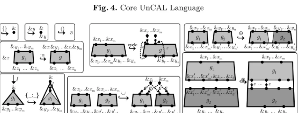
Fig. 4.Core UnCAL Language
{} & ()
∅ &y &
&y
g ε ε
cycle
g1
&x1...&xm
&x1...&xm &y1...&yn &x1...&xm
&y1...&yn
g1 g2 g1 g2
εε εε
&x1 &xm&x1 &xm
&x1 &xm
∪
... ...
...
&y1...&ym′&y′1...&y′n′ &y1 &ym′&y′1 &y′ n′ ... ...
l
g1 { g1
_:_}
&
&
l
&y1...&ym &y1...&ym &x :=
&x.&y1...&x.&ym
g1 g
&y1...&ym
...
&z1 &zn &z1...&zn
⊕
g1 g2
&x1...&xm&y1...&yn
g1 g2
&x1...&xm &y1...&yn
1 & &
m
x′… x′′&y1′…&yn′′ &x1′…&xm′′&y1′…&yn′′
ε ε
@
g1
&z1...&zk &x1 &xm
g2
... &y1 &yn
g1
... &x1 &xm
g2
... &y1 &yn
... ...
1 & &
m x′… x′′
1
& &
k z′… z′′
1 & &
m x′… x′′
Fig. 5.Graph Constructors of UnCAL
3.2 UnCAL Query Language
Graphs can be created in the UnCAL query language [5], where there are nine graph constructors (Fig. 4) whose semantics is illustrated in Fig. 5. We use hooked arrows (֒→) stacked with the constructor to denote the computation by the constructors where the left-hand side is the operand(s) and the right-hand side is the result.
There are three nullary constructors. () constructs a graph without any nodes or edges, so F[[()]] ∈ DB∅, where F[[e]] denotes the (forward) evaluation of expression e. The constructor {} constructs a graph with a node with default input marker (&) and no edges, soF[[{}]]∈DB.&yconstructs a graph similar to{} with additional output marker&yassociated with the node, i.e.,F[[&y]]∈DB{&y}.
The edge constructor{ : }takes a labelland a graphg∈DBY, constructs
a new root with the default input marker with an edge labeledl from the new root tog.I(&); thus{l:g} ∈DBY. The union g1∪g2 of graphsg1∈DBXY1 and
g2∈DBXY2with the identical set of input markersX ={&x1, . . . ,&xm}, constructs
mnew input nodes for each&xi∈ X, where each node has twoε-edges tog1.I(&xi)
andg2.I(&xi). Here,ε-edges are similar toε-transitions in automata and used to
connect components during the graph construction. Clearly,g1∪g2∈DBXY1∪Y2.
The input node renaming operator := takes a marker&x and a graph g ∈
DBYZ with Y = {&y1, . . . ,&ym}, and returns a graph whose input markers are
&x ∈ Marker, and &x.Y = {&x.&y1, . . . ,&x.&ym} for Y = {&y1, . . . ,&ym}. In
particular, whenY ={&}, the := operator just assigns a new name to the root of the operand, i.e., (&x :=g)∈DBY{&x} forg∈DBY.
The disjoint uniong1⊕g2 of two graphsg1 ∈ DBXX′ and g2 ∈ DBYY′ with
X ∩ Y =∅, the resultant graph inherits all the markers, edges and nodes from the operands, thus g1⊕g2∈DBX ∪YX′∪Y′.
The remaining two constructors connect output and input nodes with match-ing markers by ε-edges. g1@g2 appends g1 ∈DBXX′∪Z and g2 ∈DB
X′∪Z′
Y by
connecting the output and input nodes with a matching subset of markers X′,
and discards the rest of the markers, thus g1@g2 ∈ DBXY. An idiom &x′@g2 projects (selects) one input marker&x′ and rename it to default (&), while dis-carding the rest of the input markers (making them unreachable). The cycle constructioncycle(g) forg∈DBXX ∪Y withX ∩ Y=∅works similarly to @ but in an intra-graph instead of inter-graph manner, by connecting output and input nodes ofgwith matching markersX, and constructs copies of input nodes ofg, each connected with the original input node by an ε-edge. The output markers in Y are left as is.
It is worth noting that any graph in the data model can be expressed by using these UnCAL constructors (up to bisimilarity), where the notion of bisimilarity is extended toε-edges [5].
The semantics of conditionals is standard, but the condition is restricted to label equivalence comparison. There are two kinds of variables: label variables and graph variables. Label variables, denoted $l,$l1etc., bind labels while graph variables denoted $g,$g1 etc., bind graphs. They are introduced by structural recursion operator rec, whose semantics is explained below by example. The variable binderslet andllethaving standard meanings are our extensions used for optimization by rewriting [15].
We take a look at the following concrete transformation in UnCAL that replaces every labelabydand contracts edges labeledc.
rec(λ($l,$g).if$l=athen{d:&1}2
else if$l=cthen{ε:&3}4
else {$l :&5}6)($db)7
If the graph variable $db is bound to the graph in Fig. 3 (a), the result of the transformation will be the one in Fig. 3 (b). We call the first operand ofrecthe
bodyexpression and the second operand the argumentexpression. In the above transformation, the body is anif conditional, while the argument is the variable reference $db. We use $db as a special global variable to represent the input of the graph transformation. For the sake of bidirectional evaluation (and also used in our tracing in this paper), we superscribe UnCAL expressions with their code positionp∈Pos wherePos is the set of position numbers. For instance, in the example above, the numbers 1 and 2 in {d:&1}2 denote the code positions of the graph constructors&and{d:&}, respectively.
RE 7(C 5) (5,d,6) RE 7(C 6) (5,d,6)
d
RN 74 RN 73
RN 76 RN 72
RN 71
RN 75 RE 7(C 1) (1,a,2) RE 7(C 2) (1,a,2)
d
RE 7 (C 1) (2,a,5) RE 7 (C 2) (2,a,5)
d
RE 7 (C 5) (1,b,4) RE 7 (C 6) (1,b,4)
b
RE 7(C 3) (6,c,3) RE 7(C 4) (6,c,3)
ε RE 7(C 1) (3,a,5)
RE 7(C 2) (3,a,5) RE 7(C 5) (1,b,3) RE 7(C 6) (1,b,3)
b
d
&
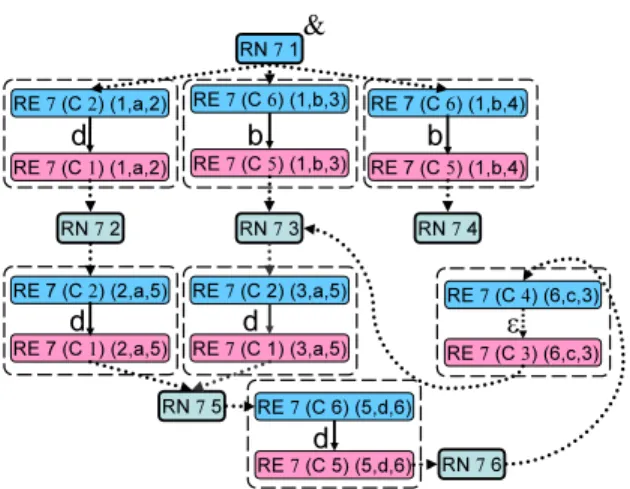
Fig. 6.Bulk semantics by example
reachable from the target node of the edge (which are correspondingly bound to variables $l and $g in the body).
In the bulk semantics, the node identifier carries some information which has the following structure [14]StrID:
StrID ::=SrcID
| Code Pos Marker
| RecN Pos StrID Marker
| RecE Pos StrID Edge,
where the base case (SrcID) represents the node identifier in the input graph,
Code p&xdenotes the nodes constructed by{},{ : },&y,∪andcyclewhere&x
is the marker of the corresponding input node of the operand(s) of the construc-tor. Except for∪, the marker is always default and thus omitted.RecN p v &z
denotes the node created by rec at position p for node v of the graph result-ing from evaluatresult-ing the argument expression. For example, in Fig. 6, the node
✄
✂RN7 1✁, originating from node 1, is created by recat position 7 (RecNis
ab-breviated to RN in the figure for simplicity, and similarly Codeto Cand RecE
toRE). We have six such nodes, one for each in the input graph. Then we eval-uate the body expression for each binding of $l and $g. For the edge (1,a,2), the result will be ({(C2),(C1)},{(C2,d,C1)},{&7→C2},{(C2,&)}), with the nodes C2 and C1 constructed by { : } and &, respectively. For the shortcut edges, anε-edge is generated similarly. Then each nodevof such results for edge
ζ is wrapped with the trace information RE like REp v ζ for recat position
p. These results are surrounded by round squares drawn with dashed lines in Fig. 6. They are then connected together according to the original shape of the graph as depicted in Fig. 6. For example, the input node✞
✝
☎
✆
connected with✄
✂RN7 1✁. After removing theε-edges and flattening the node IDs,
we obtain the result graph in Fig. 3 (b).
Our bidirectional transformation in UnCAL is based on its bidirectional evaluation, whose semantics is given by F[[ ]] and B[[ ]] as follows. F[[e]]ρ =
G is the forward semantics applied to UnCAL query e with source variable environment ρ, which includes a global variable binding $db the input graph. B[[e]](ρ, G′) =ρ′ produces the updated source ρ′ given the updated view graph
G′ and the original sourceρ.
Bidirectional transformations need to satisfy round-trip properties [7,25], while ours satisfy the GetPut and WPutGet properties [14], which are:
FJeKρ=GV
BJeK(ρ, GV) =ρ
(GetPut) BJeK(ρ, G
′
V) =ρ′ FJeKρ′=G′′V
BJeK(ρ, G′′V) =ρ′ (WPutGet)
where GetPut says that when the view is not updated after forward transforma-tion, the result of the following backward transformation agrees with the origi-nal source, and W(Weak)PutGet (a.k.a.weak invertibility[9], a weaker notion of PutGet [11] or Correctness [25] or Consistency [3] because of the rather arbitrary variable reference allowed in our language) demands that for a second view graph
G′′V which is returned byFJeKρ′, that backward transformationBJeK(ρ, G′′V) us-ing this second view graph as well as the original source environment ρ (from the first round of forward transformation) returnsρ′ again unchanged.
In the backward evaluation of rec, the final ε-elimination to hide them from the user is reversed to restore the shape of Fig. 6, and then the graph is decomposed with the help of the structured IDs, and then the decomposed graph is used for the backward evaluation of each body expression. The backward evaluation produces the updated variable bindings (in this body expression we get the bindings for $l, $g and $db and merge them to get the final binding of $db). For example, the update of the edge label of (1,b,3) in the view tox is propagated via the backward evaluation of the body {$l:&}, which produces the binding of $l updated withxand is reflected to the source graph with edge (1,b,3), replaced by (1,x,3).
UnQL as a Textual Surface Syntax of Bidirectional Graph Transformation We
(template) T ::= {L:T, . . . , L:T} | T∪T
| $g | ifBCthenTelseT
| select T where B, . . . , B
| letrec sfun fname(L: $G) =. . .infname(T)
(binding) B ::= Gp in $G | BC
(condition) BC ::= notBC | BCandBC
| BCorBC | L=L
(label) L ::= $l | a
(label pattern) Lp ::= $l | Rp
(graph pattern) Gp ::= $G | {Lp:Gp, . . . , Lp:Gp}
(regular path pat.)Rp ::= a | | Rp.Rp | (Rp|Rp)
| Rp? | Rp∗ | Rp+
Fig. 7.Syntax of UnQL
select{res:$db}
where{a:$g}in$db,
{b:$g}in$db
⇒
rec(λ($l,$g).if$l= a
then rec(λ($l′,$g).if$l′ = b
then{res:$db}
else{})($db)
else{})($db).
4
Trace-augmented forward semantics of UnCAL
This section describes the forward semantics of UnCAL augmented with explicit correspondence traces. In the trace, every view edge and node is mapped to a corresponding source edge or node or a part of the transformation. The path taken in the transformation is also recorded for the view elements.
The trace information is utilized for (1) correspondence analysis, where a selected source element is contrasted with its corresponding view element(s) by highlighting them, and likewise, a selected view element is contrasted with its corresponding parts in source and transformation, and for (2) editability analysis, classifying edges by origins to (2-1) pre-reject the editing of edges that map to the transformation, (2-2) pre-reject the conflicting editing of view edges whose edit would be propagated to the same source edge, (2-3) warn the edit that could violate WPutGet by changing branching behavior ofif by highlighting the branch conditions that are affected by the edit.
The augmented forward evaluation F[[ ]] : Expr → Env → Graph×Trace
Trace = Edge∪Node →TraceE∪TraceV
TraceE ::=Pos:TraceE|[Edge|Pos]
TraceV ::=Pos:TraceV|[Node|Pos]
The environmentEnv represents bindings of graph variables and label vari-ables. Each graph variable is mapped to a graph with a trace, while each label variable is mapped to a label with a trace that contains only edge mapping. Thus
Env =Var →(Graph×Trace)∪(Label×TraceE).
Given source graph gs and the corresponding distinct graph variable $db, the
top level environmentρ0 is initialized as follows.
ρ0={$db7→(gs,{ζ7→[ζ]|ζ∈gs.E} ∪ {v7→[v]|v∈gs.V})}
As idioms used in the following, we introduce two auxiliary functions of type
Trace →Trace: prepp to prepend code position p∈ Pos to traces, andrecep,ζ
to “wrap” the nodes in the domain of traces withRecEconstructor to adjust to bulk semantics.
preppt ={ x 7→p:τ|(x7→τ)∈t}
recep,ζt={(f x)7→ τ|(x7→τ)∈t}
wheref x=
{
(RecE p u ζ, l,RecE p v ζ) ifx= (u, l, v)∈Edge RecE p x ζ ifx ∈Node
Now we describe the semanticsF[[ ]]. The graph component returned by the semantics is the same as that of [14] and recapped in Section 3, so we focus here on the trace parts. The subscripts on the left of the constructor expressions represent the result graph of the constructions.
F[[{}p]]
ρ= (G{}p,{G.I(&)7→[p]}) (T-emp)
F[[&yp]]ρ= (G&yp,{G.I(&)7→[p]}) (Omrk)
F[[()p]]ρ= (()p,∅) (G-emp)
F[[e1∪pe2]]ρ= (G(g1∪pg2),(t1∪t2∪{v7→[p]|(&x 7→v)∈G.I}))
where ((g1, t1),(g2, t2)) = (F[[e1]]ρ,F[[e2]]ρ)
(Uni)
F[[e1⊕pe2]]ρ= (g1⊕pg2, t1∪t2)
where ((g1, t1),(g2, t2)) = (F[[e1]]ρ,F[[e2]]ρ)
(Duni)
F[[e1@pe2]]ρ= (g1@pg2, t1∪t2)
where ((g1, t1),(g2, t2)) = (F[[e1]]ρ,F[[e2]]ρ)
(Apnd)
F[[{eL :e}p]]ρ= (G{l:g}p,{(v, l, g.I(&))7→τ, v7→[p]}∪t)
where ((l, τ),(g, t)) = (FL[[eL]]ρ,F[[e]]ρ)
(Edg)
F[[(&x:=e)p]]ρ= (&x:=g, t)
where (g, t) =F[[e]]ρ
(Imrk)
F[[cyclep(e)]]ρ= (Gcyclep(g), t∪{v7→[p]|(&x 7→v)∈G.I})
where (g, t) =F[[e]]ρ
For the constructor {}, the trace maps the only node (G.I(&)) created, to the code positionpof the constructor (T-emp). The same trace information is
gen-erated for the output marker constructor (Omrk). Since neither edge nor node
is created by the constructor (), no trace information is generated (G-emp). The
binary graph constructors ∪, ⊕ and @ returns the traces of both subexpres-sions, in addition to the trace created by themselves. The graph union’s trace maps newly created input nodes to the code position (Uni). Since other two
binary constructors do not create any node or non-εedge, no additional trace is generated (Duni,Apnd). For the edge-constructor (Edg), the correspondence
between the created edge and its trace created by the label expressioneL is es-tablished, while the newly created node is mapped to the code position of the constructor. The marker-renaming expression (Imrk) does not add any trace to
that of its subexpression, since no additional node or edge is created. The cycle expression (Cyc) adds traces that map the roots created by the constructor to
the code position of the constructor.
For label expression evaluation FL[[ ]] : ExprL → Env → Label ×TraceE, the trace that associates the label to the corresponding edge or code position is accompanied with the resultant label value.
FL[[ap]]ρ= (a,[p]) (Lcnst)
FL[[$lp]]ρ= (l, p:τ)
where(l, τ) =ρ($l)
(Lvar)
Label literal expressions (Lcnst) record their code positions, while label variable
reference expressions (Lvar) add their code positions to the traces that are
registered in the environment.
Label variable binding expression (Llet) registers the trace to the
environ-ment and passes it to the forward evaluation of the body expression e. Graph variable binding expression (Let) is treated similarly, except it handles graphs
and their traces. Graph variable reference (Var) retrieves traces from the
envi-ronment and add the code position to it.
F[[lletp $l =eLine]]ρ=F[[e]]ρ∪{$l7→(l,p:τ)}
where(l, τ) =FL[[eL]]ρ
(Llet)
F[[letp $g =e1ine2]]ρ=F[[e2]]ρ∪{$g7→(g,preppt)} where(g, t) =F[[e1]]ρ
(Let)
F[[$gp]]ρ= (g,preppt)
where(g, t) = ρ($g)
(Var)
F
[[
ifp(eL=e′L)thenetrue
else efalse
]]
ρ
= (g,preppt)
where((l, ),(l′, )) = (FL[[eL]],FL[[e′L]])
b= (l=l′)
(g, t) =F[[eb]]ρ (If)
Structural recursionrec(Rec) introduces new environment for the label ($l)
by the argument expression ea, augmented with the code position pofrec. gv
denotes the subgraph of graphgthat is reachable from nodev.tvdenotes a trace
that are restricted to the subgraph reachable from nodev. The functionM takes an edge and returns the pair of the graph created by the body expressionebfor the edge, and the trace associated with the graph.tζ is the trace generated by
adjusting the trace returned byM with the node structure introduced byrec.
composep
recis the bulk semantics explained in Sect. 3.2 using Fig. 6, for the input
graph g and the input/output marker Z of eb, whereVRecN denotes the nodes
with structured IDRecN.
F[[recZ(λ($l,$g).eb)(ea)]]ρ= (g′, ∪
ζ∈g.E
tζ∪t′V)
where(g, t) =F[[ea]]ρ
M ={ζ7→ F[[eb]]ρ′ |ζ∈g.E, ζ 6=ε,(u, l, v) =ζ,
ρ′ =ρ∪{$l7→(l, p:t(ζ)),$g7→(gv,prepptv)}}
g′= (VRecN∪. . . , , , ) =composeprec(M, g,Z)
t′V ={v7→[p]|v∈VRecN}
tζ =recep,ζ(preppπ2(M(ζ)))
(Rec)
The above semantics collects all the necessary trace information whose uti-lization is described in the next section. Even though the tracing mechanisms are defined for UnCAL, they also work straightforwardly for UnQL, based on the observation that when an UnQL query is translated into UnCAL, all edge constructors and graph variables in the UnQL query creating edges in the view graph are preserved in the UnCAL query. For instance, the edge constructor
{language: $lang}and the graph variable $lang of the UnQL query in Listing
1.1 are transferred to the generated UnCAL query in Listing 1.2.
rec(λ($L,$fv1).if$L= country
then rec(λ($L,$g).if$L= name
then rec(λ($L,$fv2).if$L= people
then rec(λ($L,$e).if$L= ethnicGroup
then rec(λ($L,$lang).if$L= language
then rec(λ($L,$cont).if$L= continent
then rec(λ($l,$Any).if$l = Europe
then{result:{ethnic: $e, language: $lang, located: $cont}}
else{})($cont)
else{})($fv1)
else{})($fv1)
else{})($fv2)
else{})($fv1)
else{})($fv1)
else{})($db)
One limitation is: in our system, the bidirectional interpreter of UnCAL op-tionally rewrites expressions for efficiency. However, due to reorganization of expressions during the rewriting, we currently support neither tracing UnCAL nor tracing UnQL if the rewriting is activated.
5
Correspondence and Editability Analysis
Query
V iew Source
This section elaborates utilization of the traces defined in Sect. 4 for the correspondence and editability analysis motivated in Sect. 2. It allows us to tell the
correspon-dence between elements of the source graph, code positions of the transformation query and elements of the view graph, and editability of the edges in the view graph.
Given transformation e, environment ρ0, and the corresponding trace t for (g, t) =F[[e]]ρ0 through semantics given in Sect. 4, the trace for view edgeζhas
the following form
t(ζ) =p1:p2:. . .:pn: [x] (n≥0)
wherexis the origin, andx=ζ′∈Edgeifζ is a copy ofζ′ in the source graph, or x=p∈Pos ifζ is created of a label constant at positionpin the transfor-mation.p1, p2, . . . , pn represent code positions of variable definitions/references
and conditionals that conveyedζ.
For view graphgand tracet, define the functionorigin:Edge→Edge∪Pos
and its inverse:
origin ζ=last(t(ζ))
origin−1 x={ζ|ζ∈g.E,originζ=x}
Correspondence is then the relation between the domain and image of trace
t, and various individual correspondence can be derived, the most generic one being R : Edge∪Node ∪Pos ×Edge∪Node = {(x′, x)|(x7→τ)∈t, x′∈τ}, meaning that x′ and x is related if (x′, x) ∈ R. Source-target correspondence being {(x′, x)|(x7→τ)∈t, x′ =lastτ, x′ ∈(Node∪Edge)}. For correspondence analysis in the GUI,ζ′ is highlighted in the source graph pane, while language constructs atpfor allp1, p2, . . . , pn are highlighted in the transformation pane.
Using origin and origin−1, corresponding source, transformation and view ele-ments can be identified in both directions. When a view element such as the edgeζ= (4,German,2) in Fig. 2 is given, we can find the corresponding source
edge origin(ζ) = (1,German,0), which will be updated if we change ζ. In
con-trast, given the view edge (14,language,4), the code position of the label con-stant lang in {lang : $e} of the select part in Listing 1.1 is obtained. Given the view edgeζ = (3,German,1), the code positions of the the graph variables $lang of the select part and $db in Listing 1.1 are obtained, utilizing code positions in p1, . . . , pn, because t ζ includes such positions. These graph
ζ′ = (1,German,0) is given, we can find the set of corresponding view edges
{(3,German,1),(4,German,2)}, sinceorigin−1ζ′ is equal to this set.
For editability analysis, the following notion of equivalence is used. Given the partial function originE : Edge → Edge defined by originE ζ =
origin(ζ) if origin(ζ) ∈Edge, or undefined otherwise. Then, view edges ζ1 and
ζ2 are equivalent, denoted by ζ1 ∼ζ2, if and only iforiginEζ1 =originEζ2. All edges for which originE is undefined are considered equivalent. The equivalence class for edgeζ is denoted by [ζ]∼. Then,
1. An edit on the view edge ζwithζ′ =originEζ defined is propagable toζ′ in the source graph byB, when both of the followings hold.
(a) Other view edges in [ζ]∼ are unchanged or consistently updated.
(b) For everyifeB. . . expression in the backward evaluation path in which
eB refers a variable $l that binds label of edges originated fromζ′ (i.e.,
ρ($l) = ( , τ) and last(τ) = ζ′), applying the edit to the binding does not change the condition.
2. An edit on the view edgeζwithorigin(ζ) =p∈Pos is not propagable to the source. Editing label constant atpin the transformation would achieve the edits, with possible side effects through other copies of the label constant.
Consider the example in Listing 1.1 with the source graph of Fig. 1 and view graph of Fig. 2. We get four equivalence classes, one each for the source edges (1,German,0), (3,Europe,2), (5,Austrian,4) and (11,German,10), as well as the class that satisfy condition 2. For view edge ζ = (3,German,1), we have
(4,German,2)∈[ζ]∼ viaoriginEζ= (1,German,0), so these equivalent edges can
be selected simultaneously, inconsistent edits on which can be prevented. Direct edits of the view edge ζ = (0,result,14) are suppressed since originζ ∈ Pos
(condition 2). As for case 1b, when the view edgeζ= (7,Europe,5) is given, all the code positions int ζ′′forζ′′∈originE−1(originEζ) are checked if the positions represent conditionals that refer variables, change of those binding would change the conditions and would be rejected byB. We obtain the position for variable reference $l in the condition ($l=Europe) for warning.
Details on Branch Behavior Change Rejection in the Backward Transformation
and its Prevention Here we briefly review how updates in case 1b are rejected by
B. Given transformationeand view edgeζto be updated and the corresponding source edge ζ′ = originEζ, for each B[[if eB. . .]] invoked from B[[e]], for all bindings of label variables with the same source edge, in the condition expression
eB, label update to ζ′ is applied, and eB is reevaluated based on the updated bindings. If the reevaluation result differs from that in the forward direction, the update is rejected.
Next we explain how the case 1b is detected without conducting the entire backward transformation. SupposeoriginE−1ζ′ =E and let E′ the set of edges in E that are reachable from the roots of the view graph. For each ζ′′ ∈ E′,
variables in the condition expression. If any of the conditions change, then the condition 1b is detected and edits ofζ are prevented.
6
Our GRoundTram System
We have integrated the tracing mechanisms in the form of highlighting and editability support described above into our GRoundTram system. The imple-mentation is on our project website athttp://www.prg.nii.ac.jp/projects/
gtcontrib/cmpbx/. In the following, we summarize the new features available
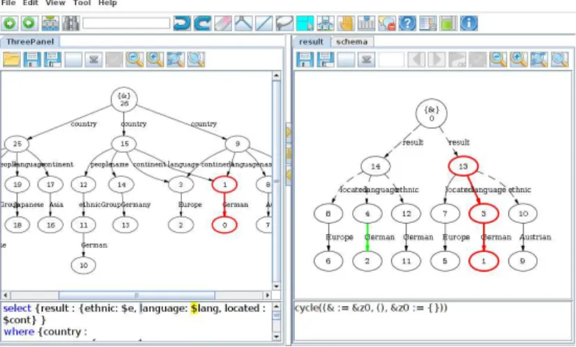
to the users. Fig. 8 shows a screenshot of GRoundTram.
Fig. 8.Screenshot of the GRoundTram system showing traces between source graph, UnQL transformation and view graph
View edges have their origins highlighted when they are selected, be it a single view edge in the selection or a whole collection of edges. Direct copies from the source graph will have their corresponding source edge highlighted, as well as the graph variable in the query that produced them. Other view edges have the relevant edge constructor highlighted in the query instead. In Fig. 8, an edge constructor with a constant label as well as a graph variable are highlighted (in different colors for the benefit of the user). In addition, several source edges are identified as the origins of direct copies that are part of the view selection.
Highlighting also works in reverse to find the copies of source edges in the view as well as the corresponding view edges for a given graph constructor or graph variable in the query.
equivalence class are highlighted in a green color (also seen in Fig 8). The system prevents inconsistent edits from happening.
7
Related Work
Tracing mechanism. Van Amstel et al. proposed a visualization framework
for chains of ATL model transformations [2]. Systematic augmentation of the trace-generating capability with model transformations is achieved by higher-order model transformations [26]. Although they also trace between source, transformation and target, we also use the trace for editability analysis. Our own previous work [14] introduced the trace generation mechanism, but the main objective was the bidirectionalization itself. The notion of traces has been extensively studied in a more general context of computations, like provenance traces [6] for the nested relational calculus.
Lifting traces from the core language to its surface language (syntactic sugar), like UnCAL to UnQL in our work, is not easy in general due to the generally big gap between the two languages. Pombrio and Krishnamurthi [23] tackle with this gap by automatically reproducing an evaluation sequence of the core language in the surface language, which may provide a partial solution for us to cope with higher level sugar likereplacein our previous work [20,17].
Triple Graph Grammars (TGG) [24] and frameworks based on them are studied extensively and are applied to model-driven engineering [1]. They are based on graph rewriting rules consisting of triples of source and target graph pattern, and the correspondence graph in-between which explicitly contains the trace information. Grammar rules are used to create new elements in source, correspondence and view graphs consistently. By iterating over items in the cor-respondence graph, incremental TGG approaches can also work with updates and deletions of elements [12]. Our transformation language UnQL is compo-sitional in that it allows arbitrary intermediate graphs to be produced in the transformation, while TGG is not. Our tracing over compositions are achieved by keeping track of variable bindings.
Editability Analysis. Another well-studied bidirectional transformation
can trace nodes (though we focused on edge tracing in this paper) while theirs cannot.
8
Conclusion
Bidirectional transformations sometimes receive a reputation that the result of backward transformation is difficult to understand or predict. This applies to frameworks like our GRoundTram system in which the backward semantics is completely provided, rather than (partially) left to the users, so the logic of backward transformation is rather fixed and hidden by the semantics. The pre-diction is even more difficult for more complex transformations. In this paper, we proposed, within a compositional bidirectional graph transformation framework based on structural recursion, a technique for analyzing the correspondence be-tween source, transformation and target as well as to classifying edges according to their editability. We achieve this by augmenting the forward semantics with explicit correspondence traces. The incorporation of this technique into the GUI enables the user to clearly visualize the correspondence. Moreover, prohibited edits such as changing a constant edge and updating a group of edges inconsis-tently are disabled. This allows the user to predict violated updates and thus do not attempt them at the first place.
As a future work, we would like to accommodate update operations other than edge renaming, like insertion of subgraphs, using the same backward transformation semantics, because we currently handle insertions using a separate general inversion strategy which is costly. We currently have lim-ited support, however we do not have bidirectional properties for complex expressions. One obvious case we can support is subgraph extraction like
select {a: $g} where {a: $g} in $db, in which we could insert an arbitrary subgraph below the top level edge labeled a. Because the subgraph is not “observed” in the transformation, an update will never interfere with the branching behavior. Even though that part is “observed” by the bulk semantics, that part is left unreachable, so the update does not affect the computation of the reachable part. Leveraging the traces in the forward semantics indicating which edge is involved in the branching behavior, we could safely determine the part that accepts the insertion or deletion of that part reusing the in-place update semantics, thus achieving “cheap backward transformation”.
We also would like to overcome the limitations of tracing UnQL with opti-mization activated by defining rules of how to pass position information of edge constructors and graph variables in an UnCAL expression to the corresponding elements in the optimized expression. Our foray in this direction shows promising results.
Acknowledgments. The authors would like to thank Zhenjiang Hu and
References
1. Amelunxen, C., Klar, F., K¨onigs, A., R¨otschke, T., Sch¨urr, A.: Metamodel-based tool integration with MOFLON. In: ICSE ’08. pp. 807–810. ACM (2008)
2. van Amstel, M.F., van den Brand, M.G.J., Serebrenik, A.: Traceability visualiza-tion in model transformavisualiza-tions with TraceVis. In: ICMT’12. pp. 152–159 (2012) 3. Bancilhon, F., Spyratos, N.: Update semantics of relational views. ACM Trans.
Database Syst. 6(4), 557–575 (1981)
4. Bohannon, A., Foster, J.N., Pierce, B.C., Pilkiewicz, A., Schmitt, A.: Boomerang: Resourceful lenses for string data. In: POPL ’08. pp. 407–419 (2008)
5. Buneman, P., Fernandez, M., Suciu, D.: UnQL: a query language and algebra for semistructured data based on structural recursion. The VLDB Journal 9(1), 76–110 (2000)
6. Cheney, J., Acar, U.A., Ahmed, A.: Provenance traces. CoRR abs/0812.0564 (2008) 7. Czarnecki, K., Foster, J.N., Hu, Z., L¨ammel, R., Sch¨urr, A., Terwilliger, J.F.: Bidirectional transformations: A cross-discipline perspective. In: ICMT’09. pp. 260–283 (2009)
8. Dayal, U., Bernstein, P.A.: On the correct translation of update operations on relational views. ACM Trans. Database Syst. 7(3), 381–416 (1982)
9. Diskin, Z., Xiong, Y., Czarnecki, K., Ehrig, H., Hermann, F., Orejas, F.: From state- to delta-based bidirectional model transformations: The symmetric case. In: MODELS’11, LNCS, vol. 6981, pp. 304–318 (2011)
10. Eramo, R., Pierantonio, A., Rosa, G.: Uncertainty in bidirectional transformations. In: Proc. 6th International Workshop on Modeling in Software Engineering (MiSE). pp. 37–42. ACM (2014)
11. Foster, J.N., Greenwald, M.B., Moore, J.T., Pierce, B.C., Schmitt, A.: Combinators for bidirectional tree transformations: A linguistic approach to the view-update problem. ACM Trans. Program. Lang. Syst. 29(3) (2007)
12. Giese, H., Wagner, R.: From model transformation to incremental bidirectional model synchronization. Software & Systems Modeling 8(1), 21–43 (2008)
13. Hidaka, S., Billes, M., Tran, Q.M.: A trace-based approach to increased com-prehensibility and predictability of bidirectional graph transformations. Tech. Rep. GRACE-TR-2015-03, GRACE Center, National Institute of Informatics (Sep
2014),http://www.prg.nii.ac.jp/projects/gtcontrib/cmpbx/cmpbx.pdf
14. Hidaka, S., Hu, Z., Inaba, K., Kato, H., Matsuda, K., Nakano, K.: Bidirectionalizing graph transformations. In: ICFP’10. pp. 205–216. ACM (2010)
15. Hidaka, S., Hu, Z., Inaba, K., Kato, H., Matsuda, K., Nakano, K., Sasano, I.: Marker-directed optimization of UnCAL graph transformations. In: LOPSTR’11, Revised Selected Papers. LNCS, vol. 7225, pp. 123–138 (Jul 2012)
16. Hidaka, S., Hu, Z., Inaba, K., Kato, H., Nakano, K.: GRoundTram: An integrated framework for developing well-behaved bidirectional model transformations (short paper). In: ASE’11. pp. 480–483. IEEE (2011)
17. Hidaka, S., Hu, Z., Inaba, K., Kato, H., Nakano, K.: GRoundTram: An Inte-grated Framework for Developing Well-Behaved Bidirectional Model Transforma-tions. Progress in Informatics (10), 131–148 (March 2013), http://dx.doi.org/ 10.2201/NiiPi.2013.10.7, journal version of [16]
19. Hidaka, S., Hu, Z., Kato, H., Nakano, K.: A compositional approach to bidirectional model transformation. In: ICSE New Ideas and Emerging Results track, ICSE Companion. pp. 235–238. IEEE (2009)
20. Hidaka, S., Hu, Z., Kato, H., Nakano, K.: Towards a compositional approach to model transformation for software development. In: Proc. of the 2009 ACM symposium on Applied Computing (SAC). pp. 468–475. ACM (2009)
21. Hidaka, S., Terwilliger, J.F.: Preface to the third international workshop on bidi-rectional transformations. In: Workshops of the EDBT/ICDT 2014. pp. 61–62.
http://ceur-ws.org/Vol-1133#paper-09
22. Matsuda, K., Wang, M.: “bidirectionalization for free” for
monomor-phic transformations. Science of Computer Programming (2014),
DOI:10.1016/j.scico.2014.07.008
23. Pombrio, J., Krishnamurthi, S.: Resugaring: Lifting evaluation sequences through syntactic sugar. In: PLDI’14. pp. 361–371. ACM (2014)
24. Sch¨urr, A.: Specification of graph translators with triple graph grammars. In: WG ’94. LNCS, vol. 903, pp. 151–163 (Jun 1995)
25. Stevens, P.: Bidirectional model transformations in QVT: semantic issues and open questions. Software and System Modeling 9(1), 7–20 (2010)
26. Tisi, M., Jouault, F., Fraternali, P., Ceri, S., B´ezivin, J.: On the use of higher-order model transformations. In: ECMDA-FA’09. LNCS, vol. 5562, pp. 18–33 (2009) 27. Voigtl¨ander, J.: Bidirectionalization for free! (pearl). In: POPL ’09. pp. 165–176.